
Published research
S&P 500 Seasonality and the U.S. Presidential Election Cycle
Summary
Historically, the S&P 500’s third presidential-term year has produced the strongest returns and win rate, while the midterm year has generated the weakest returns and deepest average intra-year drawdown. The most persistent subperiod is the fourth quarter of year 2 through the first half of year 3, but realized-volatility differences across cycle years are not statistically robust. September weakness is better supported than a bearish-October rule, and party or unified-versus-divided-government effects are highly confounded. The 2026 midterm year should therefore be interpreted through its current growth, inflation and monetary-policy regime rather than treated as a replay of the historical average. (simianx.ai)
S&P 500 Seasonality and the U.S. Presidential Election Cycle
Review period: 1872-01-01 to 2026-09-20 Scope: Historical S&P 500 presidential-cycle returns, volatility, drawdowns, monthly seasonality, political-control effects, macro-regime robustness and the 2026 midterm-year context. Source policy: Primary data, official statistics and peer-reviewed or institutional research were prioritized; market commentary was used mainly for recent calculations or independent cross-checks.
Executive summary
The strongest descriptive result is the third, or pre-election, year. In a reproducible grouping of S&P 500 total returns from 1928–2025, year 3 averaged 17.8%, had a 22.5% median return and finished positive in 92% of observations. The second, or midterm, year was weakest at a 7.1% average, 5.0% median and 58% win rate. Year 1 and year 4 occupied the middle. The ranking also survives post-1950 and post-1980 sample splits, although each modern bucket contains only about a dozen observations. (simianx.ai)
Risk evidence is more nuanced. Since 1950, year 2 has had the deepest average intra-year drawdown—about 18.5%, versus 11%–13% in the other years. However, a peer-reviewed presidential-cycle study found realized volatility of 11.5%, 13.4%, 12.5% and 12.2% in years 1–4, respectively, and could not statistically reject equal volatility across the four years. Thus, deeper midterm drawdowns are better supported than claims of a distinct, reliably higher midterm volatility regime. (hussmanfunds.com)
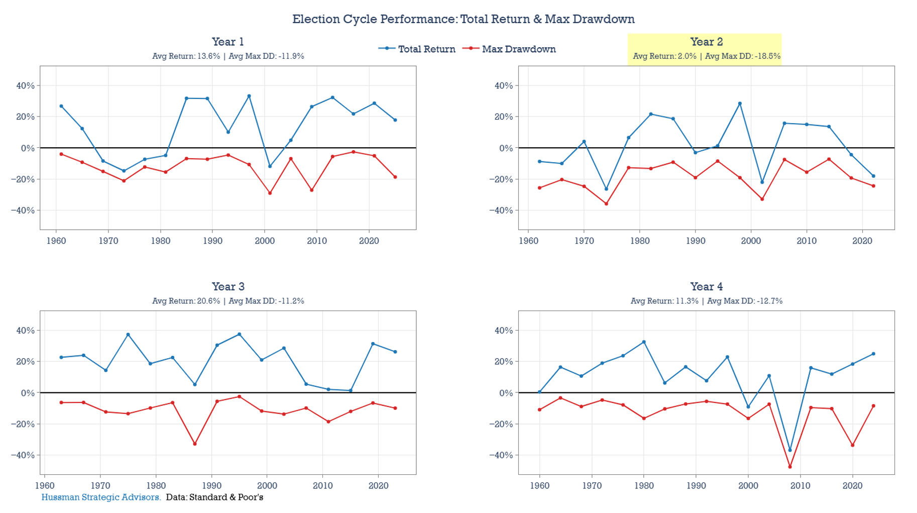
The most economically interesting subperiod is not the entire midterm calendar year but the transition from late year 2 into early year 3. Research covering 1954–2017 found average returns of 8.89%, 8.02% and 6.15% in the fourth quarter of the midterm year and the following two quarters, compounding to 24.9%; 90.9% of those quarterly observations were positive. More recent institutional calculations similarly find that markets have tended to turn roughly a month before the vote rather than immediately afterward. (ir.canterbury.ac.nz)
Monthly data support a September effect, not a simple “September–October crash” rule. September was negative on average in all four cycle years, including −1.49% in midterm years. But midterm October averaged +2.30%, followed by +2.08% in November. October has often contained a low or volatility event, yet a month can contain a sharp drawdown and still close higher. Treating October itself as predictably bearish is folklore. (gurufocus.com)
Party and government-control comparisons are much less reliable. Raw returns have historically been higher under Democratic presidents, but postwar estimates are not always statistically significant and may reflect crisis timing, oil shocks, productivity, inherited conditions and endogenous voter behavior. Likewise, recent research finding higher excess returns under unified government conflicts with the popular “gridlock is bullish” narrative, but political-control samples are small and non-random. (nber.org)
As of September 20, 2026, the current year is a Republican, second-term, unified-government midterm year. The S&P 500 had a 10.9% year-to-date price return as of September 10, but that partial-year price return is not directly comparable with full-calendar-year historical total returns. The macro backdrop—positive but slower GDP growth, 3.4% headline inflation and a September Federal Reserve rate increase—also differs from the uncomplicated policy-easing story often attached to post-midterm rallies. History supplies a distribution and a list of risks, not a forecast. (spglobal.com)
1. Method and important data qualifications
The principal long-run return comparison uses calendar-year S&P 500 total returns, including reinvested dividends, from the NYU Stern historical-return series maintained by Aswath Damodaran. Cycle position is assigned arithmetically: years divisible by four are presidential-election years; the following calendar years are years 1, 2 and 3. (pages.stern.nyu.edu)
The official S&P 500 was launched on March 4, 1957. S&P Dow Jones Indices states that index information before that launch is hypothetical and back-tested. Results beginning in 1928—and especially reconstructions extending to 1872—should therefore be understood as broad large-cap U.S. equity histories rather than live contemporaneous S&P 500 performance. (spglobal.com)
Three different risk concepts should not be confused:
- Realized volatility: annualized variability calculated from daily returns.
- Cross-year dispersion: the standard deviation of annual calendar returns within a cycle bucket.
- Maximum drawdown: the largest peak-to-trough decline within a calendar year.
These measures can disagree. A year can have moderate average realized volatility but one deep, short-lived drawdown, or high day-to-day volatility without a severe net loss.
2. Core historical measurements
The following table combines the most recent long-run total-return calculation with separate realized-volatility and drawdown studies. The columns do not share identical sample periods, so they should be read as triangulation rather than one homogeneous dataset.
| Presidential-cycle year | Avg. total return, 1928–2025 | Median | Positive years | Annualized realized volatility, 1948–2008 | Avg. maximum drawdown, since 1950 |
|---|---|---|---|---|---|
| Year 1 — post-election | 10.6% | 12.4% | 60% | 11.5% | −11.9% |
| Year 2 — midterm | 7.1% | 5.0% | 58% | 13.4% | −18.5% |
| Year 3 — pre-election | 17.8% | 22.5% | 92% | 12.5% | −11.2% |
| Year 4 — presidential election | 11.9% | 15.9% | 84% | 12.2% | −12.7% |
Return and win-rate calculations are based on 24 or 25 years per bucket. Realized-volatility differences were not statistically significant in the cited study; the drawdowns are descriptive averages. (simianx.ai)
Interpretation by year
- Year 1: The long-run reputation for weakness is overstated. Its 10.6% average is close to the unconditional average, and since 1980 year 1 has averaged 18.3% with an 83% win rate. Much of its weak reputation comes from losses clustered before 1982. (simianx.ai)
- Year 2: It has the lowest mean, median and win rate, plus the deepest typical drawdown. This is the most defensible “weak year” characterization, although the calendar-year return has still been positive more often than negative. (simianx.ai)
- Year 3: It has the strongest average, median and win rate. Since 1950, every completed year 3 has finished positive, averaging 20.8%. The two negative full-sample observations were 1931 and 1939. (simianx.ai)
- Year 4: Presidential-election years have been positive 84% of the time, but the 11.9% average is not dramatically different from the market’s unconditional long-run average. The 2008 financial crisis demonstrates that election-year incentives do not override the business or credit cycle. (simianx.ai)
Sensitivity to the chosen historical period
| Cycle year | Since 1928 | Since 1950 | Since 1980 |
|---|---|---|---|
| Year 1 | 10.6%; 60% up | 11.5%; 63% up | 18.3%; 83% up |
| Year 2 | 7.1%; 58% up | 8.3%; 63% up | 5.9%; 64% up |
| Year 3 | 17.8%; 92% up | 20.8%; 100% up | 19.2%; 100% up |
| Year 4 | 11.9%; 84% up | 11.4%; 89% up | 10.0%; 83% up |
The stability of year 3’s ranking is notable. Year 1, however, changes character dramatically in the modern era, while year 2 remains weak but has a slightly better modern win rate. (simianx.ai)
A much longer 1872–2020 reconstructed price-return series produces lower absolute averages—4.4%, 3.9%, 10.3% and 6.1% for years 1–4—but preserves the same broad ordering. Its annual-return standard deviations were 19.8%, 16.9%, 19.3% and 16.6%, respectively. Thus, year 2 did not have the greatest cross-year dispersion even though it had the deepest average drawdown in the post-1950 drawdown study. (readkong.com)
3. Monthly seasonality inside the four-year cycle
The table below reports published long-sample average monthly returns. Because the underlying webpage does not fully document adjustments and index reconstruction, these figures are most useful for identifying the shape of seasonality rather than estimating a tradable premium.
| Month | Year 1 | Year 2: midterm | Year 3 | Year 4 |
|---|---|---|---|---|
| January | 0.84% | 0.50% | 3.52% | 0.08% |
| February | −1.65% | −0.03% | 1.40% | −0.10% |
| March | 0.35% | −0.27% | 0.69% | 0.92% |
| April | 2.32% | 0.83% | 2.51% | −0.18% |
| May | 2.07% | −0.53% | −0.15% | −0.89% |
| June | 0.74% | −1.31% | 2.25% | 1.52% |
| July | 2.27% | 0.96% | 1.32% | 2.12% |
| August | 0.13% | −0.33% | −0.10% | 3.06% |
| September | −1.41% | −1.49% | −1.24% | −0.36% |
| October | −0.47% | 2.30% | 0.71% | −0.37% |
| November | 0.65% | 2.08% | −0.11% | 1.32% |
| December | 0.52% | 0.86% | 2.33% | 1.35% |
Source for the monthly matrix: (gurufocus.com)
What the monthly pattern actually says
September weakness is broad rather than election-specific. It is negative in every cycle position and is especially weak in years 1–3. Across all years in the same dataset, September averaged −1.12%. (gurufocus.com)
Midterm weakness is concentrated before October. May, June, August and September were all negative on average in year 2. October and November were among year 2’s strongest months. Nasdaq Dorsey Wright’s updated 1928–2026 calculation similarly found that only 44% of midterm first quarters were positive, increasing to 83.3% in fourth quarters. (gurufocus.com)
“October is bad” confuses volatility with return. October contains several famous crashes and has often marked an intra-year trough. But the average midterm October return was positive. A sharp early-October decline followed by a larger recovery can produce both an “October low” and a positive monthly return.
Year 3 strength is front- and back-loaded. January, April, June and December have historically done most of the work. September remained weak even in the strongest cycle year. (gurufocus.com)
4. Midterms and the post-midterm rally
Evidence for the pattern
A Journal of Wealth Management study of the S&P 500 Total Return Index over 1954–2017 found:
- Fourth quarter of the midterm year: 8.89% average return.
- First quarter of year 3: 8.02%.
- Second quarter of year 3: 6.15%.
- Three-quarter compounded return: 24.9%.
- Positive observations: 90.9%.
- Annualized volatility in the post-midterm window: 12.7%, versus 15.4% in non-election periods.
The study reported similar means and medians, making a single extreme winner an unlikely explanation for the result. It also concluded that the late-year-2/early-year-3 window was stronger than the generic full-calendar-year “year 3 effect.” (ir.canterbury.ac.nz)
Updated institutional evidence points in the same direction but with smaller magnitudes. BlackRock found an average 14.1% total return in the six months after midterms since 1970, with the turn historically beginning about 22 trading days before Election Day. J.P. Morgan reports slightly negative average returns in each of the first three midterm-year quarters and an average 6.6% gain in the fourth quarter. (blackrock.com)
Why it may exist
Plausible mechanisms include the resolution of policy uncertainty, reduced probability of major legislation after the president’s party loses seats, mean reversion from a weak midterm drawdown and a coincident shift in monetary or economic conditions. These mechanisms are not mutually exclusive.
The timing is important: if the average recovery begins before the election, “wait until the result is known” is not the historical strategy being measured. It is also evidence that the effect may reflect anticipatory pricing rather than a mechanical response to the announced result. (blackrock.com)
Reasons for caution
There have been only about 18–24 usable midterm episodes, depending on the starting date. Fixed 6- or 12-month post-election windows overlap with the structurally strong year 3, making it difficult to determine whether the event is the election, the cycle position, mean reversion or the macro environment.
Claims such as “stocks have never fallen in the 12 months after a midterm” are extremely sensitive to the exact start date, index definition and sample start. Even when historically correct for a chosen dataset, zero failures in roughly 19 observations does not imply zero future probability.
5. Democratic versus Republican administrations
Raw historical averages show a large Democratic advantage. First Trust calculates average annual S&P 500 total returns of 14.98% under Democratic presidents and 7.84% under Republican presidents from 1929–2025. CRSP-based academic research for 1927–2015 found annual excess returns of 10.7% under Democrats and −0.2% under Republicans. (ftportfolios.com)
The party difference also appears within the long 1872–2020 cycle reconstruction: Democratic administrations had higher average returns in years 1, 2 and 3, while Republican administrations were slightly ahead in year 4. However, splitting four cycle positions by two parties leaves only approximately 8–12 observations in many cells. (readkong.com)
Why the raw party gap is not a causal estimate
Blinder and Watson’s postwar economic study found S&P 500 returns averaging 8.35% under Democrats and 2.70% under Republicans, but the 5.65-percentage-point difference had a p-value of 0.15. Their broader economic analysis attributed the Democratic macroeconomic advantage largely to more favorable oil shocks, productivity developments, international conditions and possibly expectations—not simply to presidential policy. (swh.princeton.edu)
Pástor and Veronesi provide an endogenous-risk explanation: economic crises raise risk aversion and demand for social insurance, which makes Democratic victories more likely at times when expected equity premia are high. Under that interpretation, political affiliation partly reflects the economic state rather than independently causing subsequent returns. (nber.org)
Assessment: The Democratic return premium is a real historical sample fact, but it is not a reliable stand-alone causal or forecasting variable. Its economic magnitude is more convincing than its attribution to party policy.
6. Unified versus divided government
Popular commentary often claims that markets prefer divided government because gridlock limits disruptive policy. The empirical record is not that simple.
A recent 94-year CRSP study reports annualized value-weighted excess returns of 10.3% under unified government and 1.6% under divided government—an 8.7-percentage-point statistically significant difference. The authors report robustness to outliers and persistence and find that presidential-party affiliation loses explanatory power when unified-versus-divided status is included. This is a recent working paper rather than a settled consensus, however. (aeaweb.org)
J.P. Morgan’s simpler S&P 500 comparison since 1937 shows 16.3% average returns under unified Republican control versus 9.4% under a Republican president with divided Congress. J.P. Morgan explicitly warns that fiscal, monetary, growth, profit and valuation conditions are more informative than the political labels themselves. (am.jpmorgan.com)
Around midterms, BlackRock finds that a unified government losing its trifecta was followed by a 10.4% average six-month return, versus 16.1% when control was gained or Congress remained divided. All of these subgroup estimates contain very few elections and should not be used to rank future political outcomes mechanically. (blackrock.com)
Assessment: “Divided government is bullish” is folklore, not a robust universal finding. Unified-government results may be stronger in some samples, but endogeneity is severe: unified control tends to occur after landslide elections and during particular economic regimes.
7. Macroeconomic regimes and confounding
Depression, postwar and modern samples
The year-3 result survives removal of the prewar period and becomes stronger after 1950. This is meaningful evidence against the claim that its average is created by one or two early observations. However, the postwar sample also overlaps with long expansions, disinflation after the early 1980s and generally rising equity valuations. With only 24 full-sample year-3 observations, those effects cannot be cleanly separated. (simianx.ai)
The 1931 crash is actually a negative year-3 outlier. Removing it raises rather than lowers the year-3 average. Conversely, the midterm average is helped by the 52.6% return in 1954; its 5.0% median is therefore a more conservative estimate of a typical midterm year. (simianx.ai)
Business-cycle and interest-rate controls
Research using 1948–2008 data found excess returns of approximately −1.0%, −4.7%, +12.6% and +1.5% in years 1–4. Tests rejected equal returns across the four years, and the pattern survived controls for dividend yield, default spread, term spread and relative interest rates. Yet the same research found no significant realized-volatility differences and could not validate the popular explanation that administrations systematically manipulate fiscal, monetary or tax policy to produce the cycle. (researchgate.net)
This creates an important distinction: evidence that a return pattern survives a set of controls is not evidence that the political-calendar mechanism commonly offered for it is correct.
Recession timing
Year 3 has contained relatively few recessions, while several large year-2 and year-4 losses occurred during recessions, credit contractions or monetary tightening. This mechanically raises year-3 averages and lowers year-2 and year-4 results. Calendar position may therefore partly summarize the historical timing of recessions rather than constitute an independent return driver. (files.advisorperspectives.com)
8. Statistical and economic significance
What looks statistically or economically meaningful
- Year 3 versus year 2 returns: The gap is large economically, persists across major sample splits and has appeared in formal postwar regressions. This is the strongest full-year result. (simianx.ai)
- Midterm drawdowns: An average maximum drawdown near 18.5%, compared with roughly 11%–13% elsewhere, is large enough to matter for portfolio risk even when the full year finishes positive. (hussmanfunds.com)
- Late-year-2 through mid-year-3 returns: This is supported by both peer-reviewed work and more recent institutional datasets and appears stronger than a generic post-election-day effect. (ir.canterbury.ac.nz)
- September weakness: It appears across all four cycle positions and in the unconditional monthly average. Its economic size is modest relative to normal market volatility, however. (gurufocus.com)
What does not survive scrutiny as well
- A unique midterm volatility premium: Year 2’s realized volatility was highest descriptively, but formal tests did not establish significant differences across cycle years. (citeseerx.ist.psu.edu)
- October as an inherently bearish month: The midterm-year average is positive; October is better described as a potential trough or high-range month.
- Party as a causal return factor: Raw gaps are large, but statistical significance, attribution and out-of-sample stability depend heavily on the sample and macro controls. (federalreserve.gov)
- Gridlock as automatically bullish: Both unified and divided government have led in different samples. (am.jpmorgan.com)
- Guaranteed post-midterm or year-3 gains: The sample is too small to justify certainty, and 1931 shows that a severe macro shock can overwhelm even the strongest seasonal bucket. (simianx.ai)
Data-mining considerations
Testing 12 months across four cycle years already creates 48 seasonal cells. Adding party, first-versus-second terms, unified-versus-divided government, incumbent status and macro regimes rapidly generates hundreds of possible comparisons. Without pre-specified hypotheses or multiple-testing adjustment, some apparently striking cells should arise by chance.
The presidential-cycle pattern was publicized in the 1960s. Year 3 has remained strong afterward, which is encouraging from an out-of-sample perspective, but the post-publication sample contains only about 15 cycles and coincides with favorable structural changes in U.S. equity markets. (simianx.ai)
Economic significance also differs from market-timing usefulness. Holding only year-3 periods generated far less terminal wealth than remaining invested through the full 1928–2025 period, because an investor following the calendar rule forfeited three-quarters of the market’s compounding and dividends. (simianx.ai)
9. Placing 2026 in the historical framework
Political position
2026 is year 2 of President Donald Trump’s second, nonconsecutive term, with the midterm election scheduled for November 3, 2026. As of August 12, Republicans held the presidency, 53 Senate seats and 219 House seats, versus 212 House Democrats and four vacancies—placing the year in the unified-Republican-government category entering the election. (simianx.ai)
Second-term year-2 comparisons illustrate the danger of excessive slicing. A reconstructed series since 1872 puts second-term year-2 returns at 13.1% overall; Republican second-term year-2 returns averaged 7.1% and were positive 83.3% of the time—but that Republican estimate contains only six observations. Goldman Sachs reports an 11.6% average price return for second-term year 2 since 1873. These figures provide context, not a dependable conditional forecast. (readkong.com)
Market position
As of September 10, the S&P 500 had a 10.9% year-to-date price return, after being up 12.28% through August 31; September-to-date was −1.23% at the September 10 observation. That places 2026 above the 7.1% full-year historical midterm total-return average at that snapshot, but the comparison mixes a partial-year price return with full-year total returns and is therefore only directional. (spglobal.com)
Macroeconomic position
Real GDP grew at a 1.5% annual rate in the second quarter, down from 2.1% in the first quarter. August CPI inflation was 3.4% year over year, while core CPI was 2.4%. On September 16, the Federal Reserve raised its target range by 25 basis points to 3.75%–4.00%, saying inflation remained elevated while economic activity continued to expand. (bea.gov)
This backdrop matters more than the label “midterm year.” Historical midterm rallies occurred under easing, tightening, recessionary and expansionary conditions. The 2026 combination of positive growth, renewed policy tightening, energy-driven headline inflation and elevated geopolitical uncertainty is not captured by one historical average.
Appropriate interpretation
For 2026, history supports three observations—not predictions:
- The late-summer/early-autumn period of a midterm year has historically carried elevated drawdown risk and weak September seasonality.
- The market has often turned before, rather than after, Election Day, making the historical path difficult to time.
- Current returns, monetary policy, valuations and growth conditions can dominate the calendar pattern, just as they did in 2002, 2018 and 2022. (blackrock.com)
10. Bottom line: evidence versus folklore
| Claim | Assessment |
|---|---|
| Year 3 is historically strongest | Robust descriptive evidence; economically large, but based on only 24 full-sample observations |
| Year 2 is historically weakest | Robust on return, win rate and drawdown; less robust as a realized-volatility claim |
| September is weak | Broadly supported across all four cycle years, but modest relative to normal volatility |
| October is bearish | Folklore; October is often a trough/high-range month, but midterm October averaged positive |
| Stocks rally after midterms | Strong historical pattern, especially from Q4 of year 2 through Q2 of year 3; exact timing varies |
| Democrats are better for stocks | Large raw historical gap, weak causal identification |
| Markets prefer divided government | Not robust; contradicted by some long-sample research |
| Election-cycle averages forecast 2026 | Unsupported; they are low-resolution priors, not forecasts |
The most defensible conclusion is that the presidential cycle contains a genuine historical asymmetry: year 2 has tended to deliver the worst path, while late year 2 through year 3 has delivered the strongest path. The evidence is materially weaker for explanations based on party, electoral engineering, gridlock or a mechanically bearish October. In practical analysis, the cycle should be subordinate to valuation, earnings, recession risk, inflation and monetary policy.
Sources
- NYU Stern historical annual total-return dataset, used for the 1928–2025 return history. (pages.stern.nyu.edu)
- S&P Dow Jones Indices, for the index launch date, pre-launch back-test qualification and 2026 index snapshot. (spglobal.com)
- Kräussl et al., Washington Meets Wall Street, for formal return, realized-volatility and macro-control tests. (citeseerx.ist.psu.edu)
- Białkowski and Marsh, Midterm Elections’ Stock Market Surge, for the late-year-2/early-year-3 evidence. (ir.canterbury.ac.nz)
- Santa-Clara and Valkanov, and Pástor and Veronesi, for the presidential-party literature. (r.jordan.im)
- Blinder and Watson, for postwar macroeconomic and party comparisons. (aeaweb.org)
- J.P. Morgan and BlackRock, for updated midterm, political-control and post-election calculations. (blackrock.com)
- Bureau of Labor Statistics, Bureau of Economic Analysis and Federal Reserve for the September 2026 macroeconomic context. (bls.gov)
Sources
- The Presidential Cycle: S&P 500 Returns by Year, 1928-2025
- www.hussmanfunds.com
- JWM-Bialkowski.indd
- Presidential Cycles, Political Parties and Monthly Stock Market Returns - GuruFocus.com
- Political Cycles and Stock Returns
- S&P 500® | S&P Dow Jones Indices
- pages.stern.nyu.edu
- The only thing we have to fear is the lack of fear itself - Merrill Lynch
- Midterm Elections and Stock Market Trends | BlackRock
- www.ftportfolios.com
- Presidents and the U.S. Economy:
- www.aeaweb.org
- 2026 Midterm Election Hub | J.P. Morgan Asset Management
- (PDF) Washington Meets Wall Street: A Closer Examination of the Presidential Cycle Puzzle
- Record Stock Valuations, Fed Independence, and Macro Volatility - Hussman Funds - Commentaries - Advisor Perspectives
- Washington Meets Wall Street:
- The Fed - Alternative Estimates of the Presidential Premium
- Gross Domestic Product | U.S. Bureau of Economic Analysis (BEA)
- The Presidential Puzzle: Political Cycles and the Stock Market
- Presidents and the US Economy: An Econometric Exploration - American Economic Association
- Consumer Price Index News Release - 2026 M08 Results